In this tutorial, we will learn how to use SUMIF function in MS Excel. This function adds the values in a range that meet a specified criteria or condition. Microsoft Excel 2021 is used.
Syntax
=SUMIF( range, criteria, sum range)
This function has three arguments.
- Range: The set of the cells which are to be evaluated against the given criteria or condition.
- Criteria, it is the condition to which range is compared. It can be a cell reference, number, expression or a function which defines the values to be added.
- For the criteria, add a question mark(?) to match a single character, asterisk(*) to match sequence of characters, add tilde(`) if you want to match actual question mark or asterisk character.
- Sum Range: This is the cell range which will be added in case criteria is matched.
Range and Criteria are required, while Sum Range is optional. Range and Sum Range should have same size.
SUMIF function has three arguments, but it can also work with two arguments. We can choose not to write the third argument, the Sum Range, then the SUMIF function applies the criteria to the Range in the first argument.
This is demonstrated in the two examples below.
Example 1: Adding values using SUMIF function
In this example, we will only use two arguments for the SUMIF function. We will be added prices of the different products. If the price of the product is above $20, it will be added.
Following data will be used.
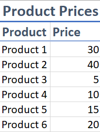
We have prices of different products, for this example, we want to add the product prices that are above $20.
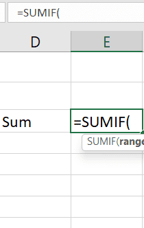
First, we enter the SUMIF formula, enter, =, before starting a formula and type SUMIF(.
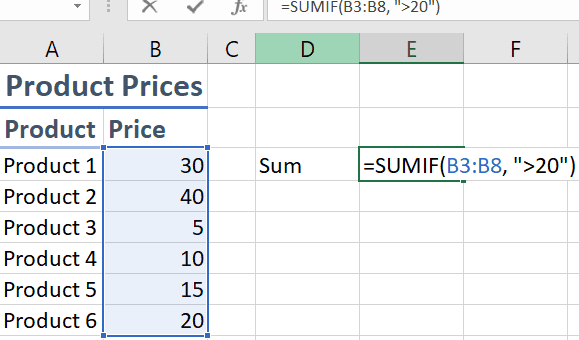
First select the range or enter it manually, and then the criteria, in this condition ">20". Remember, there should not be any spaces.
The formula becomes: =SUMIF(B3:B8,">20)
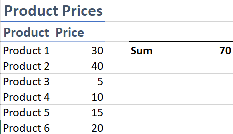
Press Enter to finalize the formula.
Example 2: Adding values of one category only using SUMIF function
For this example, we will be using all three arguments of the function. We will be adding all the prices of the fruits. The first range, will be compared if its value is “Fruit”, if yes, then add the corresponding value in the sum range.
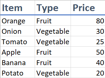
The column, Type will be range that will be checked if it has the value “Fruit”, then the corresponding value from the Price column will be added.
Enter SUMIF formula: =SUMIF(
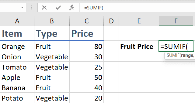
Select the range, or enter it manually, B10:B15, followed by criteria "Fruit"
Formula becomes: =SUMIF(B10:B15,"Fruit"
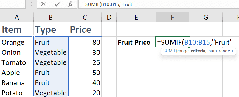
The Range and Sum Range should be equal, so, in our case, if the first item is “Fruit”, 80 is added, the second item is not a food, so it is not added.
For the third argument, select the Sum Range, which is Price for this example.
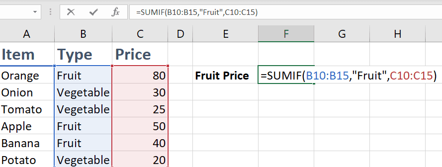
Press Enter to finalize the formula.
We have also added the price of Vegetable.


