In this tutorial, we will learn how to use TRANSPOSE function and copy, paste & transpose to switch rows and columns. By doing this, we can rotate rows and columns. Microsoft Excel 2021 is used.
We can transpose using two methods.
- By using Copy, Paste and Transpose option.
- By using Transpose function.
Copy, Paste and Transpose
With this method, rows and columns can easily be rearranged. The formatting of the new data is same as the original.
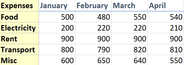
We will rearrange the following data:

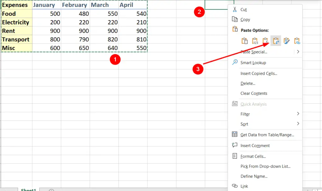
Select all the data, press CTRL+C, to copy it, select the cell where the data should be pasted, press Right Mouse Button, and click Transpose under the Paste Options.

The following image shows that the data is transposed, the rows and the columns are switched.

This method makes duplicated data, to avoid this, TRANSPOSE function is used.
TRANSPOSE function
This method is used to avoid duplicated data. This method does not copy the formatting of the cells of the original data.
We will be using the same data, for this method, you have to select blank cells, where you will use the TRANSPOSE function. Remember, select the same number of cells as the original set of cells, but they should be rotated.

Now, with all the selected cells, type the formula, =TRANSPOSE(, next specify the cells that need to be rotated, for this tutorial, they are A1:E6.
So, the formula becomes, =TRANSPOSE(A1:E6)

To apply the formula, press CTRL+SHIFT+ENTER, as it as an array formula.

As it can be seen that, this formula does not copy the formatting of the cells.

