In this tutorial, we will learn how can we use SWITCH function in MS Excel, SWITCH function checks the value of a cell against another value and returns a corresponding specified value. Microsoft Excel 2021 is used.
Syntax
Syntax of SWITCH function: = SWITCH (Value to switch, Value to check, Value to return if there is a match, ... ,Value to return if there is no match)
- In the first argument, we specify the value which needs to be switched or replaced, this is usually a cell that contains the value.
- In the second argument, we match the value against the first value.
- In the third argument, if there is match, the entered value in this argument is returned.
- In the last argument, we specify the value to return if there is no match with any value.
You may also specify the value to return if there is no match.
Example of Switch function
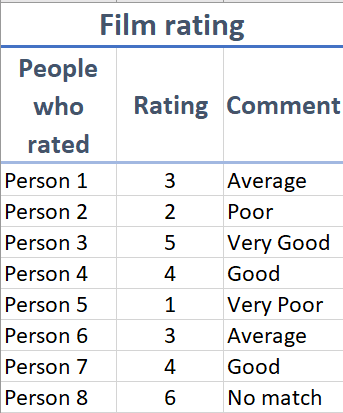
For this tutorial, we will use an example of Film ratings and how they may be considered as good or bad.
We will be using the following scheme:
| Rating | Explanation |
| 1 | Very Poor |
| 2 | Poor |
| 3 | Average |
| 4 | Good |
| 5 | Very Good |
Following data will be used.
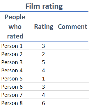
The result should appear in the “Comment” column, so that’s where the formula will be entered.
Enter the formula, =SWITCH(, and then following the syntax, we specify the cell for which the value is to be replaced, in this case, B3.
Enter: =SWITCH(B3,
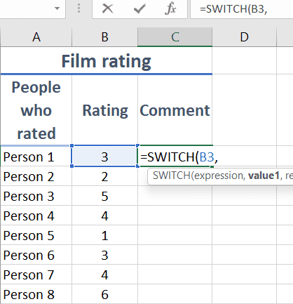
Put comma for the next argument.
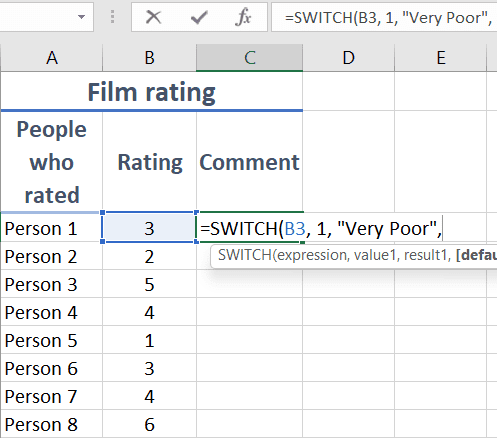
For the next two arguments, enter the value that will be matched and the result to return in case the value is matched, if not, next values will be checked
So, in case, the value is 1, return "Very Poor".
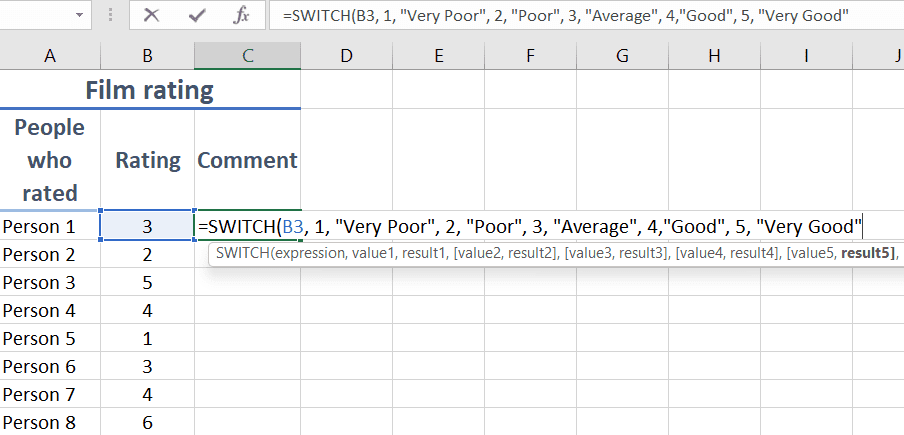
The formula becomes: =SWITCH(B3, 1, "Very Poor",
Similarly, enter the next set of values, first the value that needs to matched and the return result if the value is true.
So, the formula becomes: =SWITCH(B3, 1, "Very Poor", 2, "Poor", 3, "Average", 4,"Good", 5, "Very Good",
Now, finally, we enter the value if none of the values match. For this, we enter the result in the last argument.
So, the formula becomes: =SWITCH(B3, 1, "Very Poor", 2, "Poor", 3, "Average", 4,"Good", 5, "Very Good", "No match")
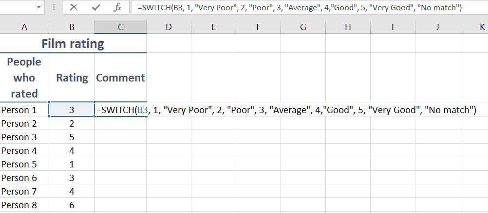
Press Enter to apply the formula.
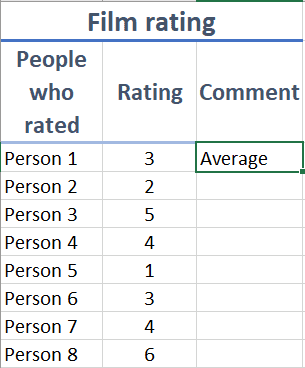
To apply the formula along the column, select the cell, drag the bottom right corner of the cell along the column.