In this tutorial, we will learn how can we use Nested If function. Basically, we use a function as the argument of another function which we refer to as nesting and the function is Nested function. For this tutorial, we will make a grading system using Nested IF function. MS Excel 2021 is used.
The IF function uses three arguments, the logical condition, value in case the result is true, and the value in case the result is false. For the Nested IF function, we will use another IF for the argument if the condition is false. Click here to check IF function tutorial.
Syntax:
IF(logical condition, [value if true], IF(...))
We will learn how can we make a grading system in Excel using Nested IF function.
Following scheme will be implented:
| Marks | Grade |
| > 90 | A+ |
| > 80 | A |
| > 70 | B |
| > 60 | C |
| > 50 | D |
| < 50 | F |
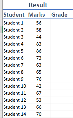
We will be using the following data for the grades and Nested IF function.
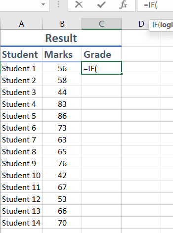
Select the cell, enter the formula starting with =IF(.
For the first condition, we need to check if the marks are above 90, and if this condition is true, the grade will be “A+”.
In our case B3 is the cell which will be checked for the IF function, if you select the cell, it will automatically enter the position of the selected cell.
Write, =IF(B3>90, "A+"
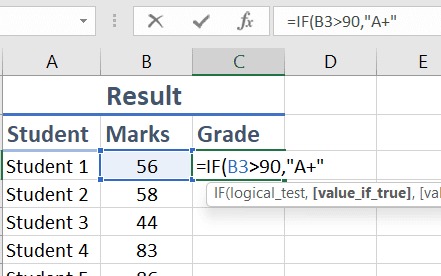
You can also type the cell position manually.
Now, if the value is false, we use another IF function as the argument of the other IF function. The new IF function will be checked in case the previous IF function is false.
The new IF function will check if the marks are above 80 if it’s true, the student will have “A” grade.
So, we enter, =IF(B3>90, "A+", IF(B3>80, "A"
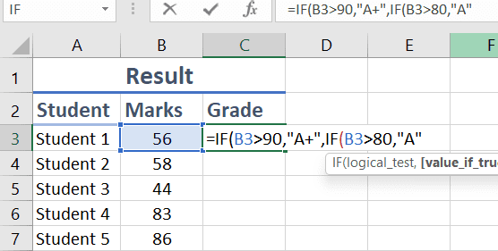
The function can be extended in the same way for B,C,D and F grades.
The function formula becomes
=IF(B3>90,"A+",IF(B3>80,"A",IF(B3>70,"B",IF(B3>60,"C",IF(B3>50,"D","F")))))
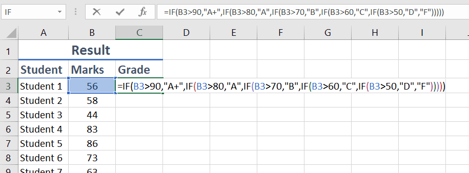
After entering the formula press Enter.
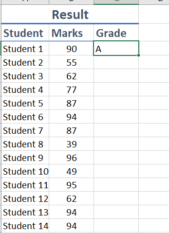
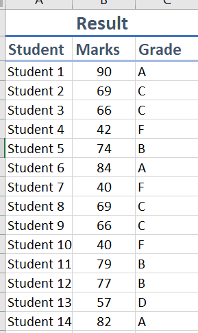
To extend the formula along the column, select the cell, drag the bottom right corner along the column.
Check out more:
