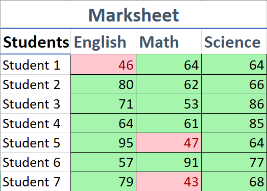
In this tutorial, we will learn how to highlight cells using Conditional Formatting. Conditional Formatting is based on a specified condition, when that condition is true, the appearance of the cell changes. MS Excel 2021 is used.
Students Marksheet will be used as an example in this tutorial. Cells that contain marks less than 50 will appear Red, while others will appear Green.
Two rules will be applied for Conditional Formatting, one for those cells which have a value less than 50, second for those cells that have a value equal to or greater than 50.
We will use following data.
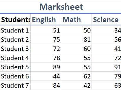
Conditional Formatting cells with value less than 50
First, the cells that have marks less than 50 will be formatted.
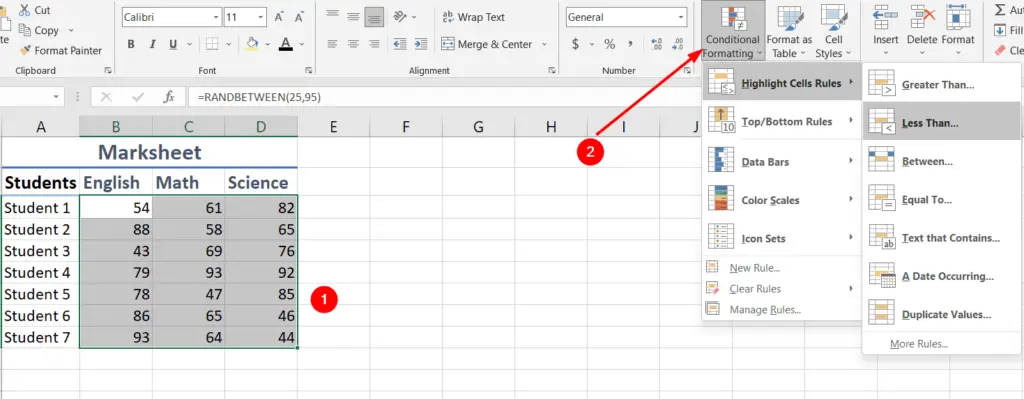
Select all the cells that need formatting. Click Conditional Formatting > Highlight Cells Rules > Less Than… from Styles on Home tab,
Less Than dialog box will appear, enter 50 in Format cells that are LESS THAN, and choose Light Red Fill for this tutorial.

All the cells that have a value less than 50 will be formatted.
Conditional Formatting cells with value equal to or greater than 50
Now, we will apply Conditional Formatting for cells having value equal to or greater than 50.
Select Conditional Formatting > Highlight Cells Rules > More Rules.
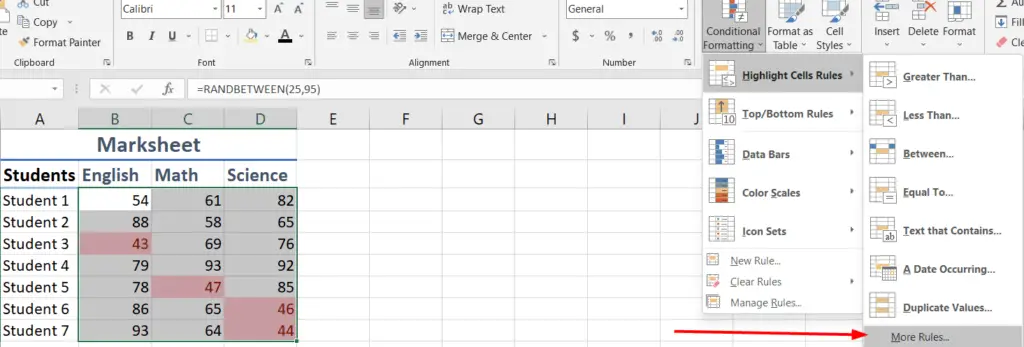
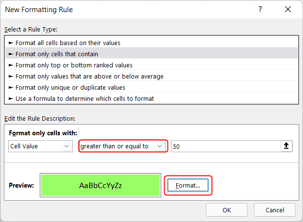
Select the condition, greater than or equal to, choose the value to be 50 and format the cell.
Manage Rules for Conditional Formatting
You can change the format of the cells which have rules applied to them using Manage rules.
To format the cells again with the applied rules, click Conditional Formatting > Manage rules.
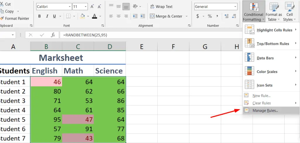
By managing rules, changes can be made to the already applied rules.
In the image below, we can see that border has been added by using Manage Rules.
