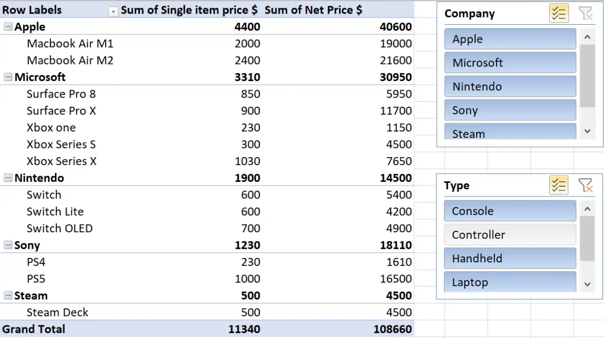
Slicers are used in Excel to filter data, they are used on Tables or PivotTables. Slicers not only filter data, but they also show what data has been filtered and what is being shown. Microsoft Excel 2021 is used.
Slicer also help visualize and understand what type of information is being displayed on the Table or PivotTable.
Slicers can only be used on a Table or a PivotTable, if you do not have either of those, click here to learn about PivotTables.
Creating Slicer
For this tutorial, we are going to use Slicer on a PivotTable.
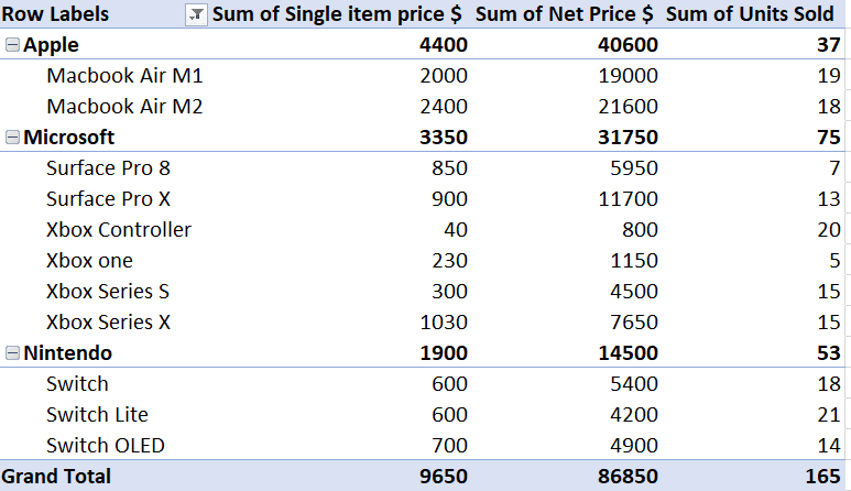
But we will create a Slicer for both PivotTable and a Standard Table.
Creating Slicer for PivotTable
To Create a Slicer for PivotTable select the PivotTable and click PivotTable Analyze > Insert Slicer.

Creating Slicer for Table
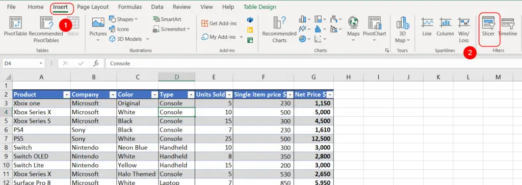
To create a Slicer for a table, select the table, and click Insert > Filters > Slicer.
Using Slicer
A menu will appear, select the parameters you wish to display and the unselected parameters will not be displayed as Slicer.
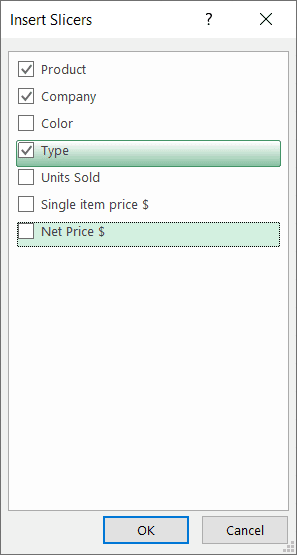
For this tutorial, we have only selected Type and Company.
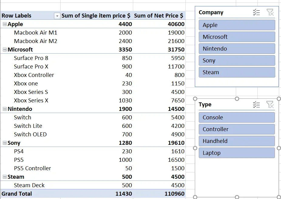
Note that, we are using two Slicers for this tutorial for our own convenience, you may use only one or more.
If you select on any of the items on the Slicer, only that item will be shown and the others will be filtered out.

In the above image, we have only selected Microsoft, so only Microsoft Products are being shown while the others have been filtered.
Multi-Select in Slicer
It it possible to select more than one item in Slicer, click on the Multi-Select button, and select multiple items.
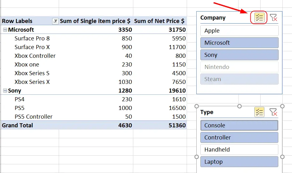
By using this feature, Multiple items are selected and shown in the PivotTable while the others are filtered out.
Clear Filter
We can clear all the filters that we have applied on a Slicer. This will reset the Slicer in its original state. Click on the Clear Filter button.
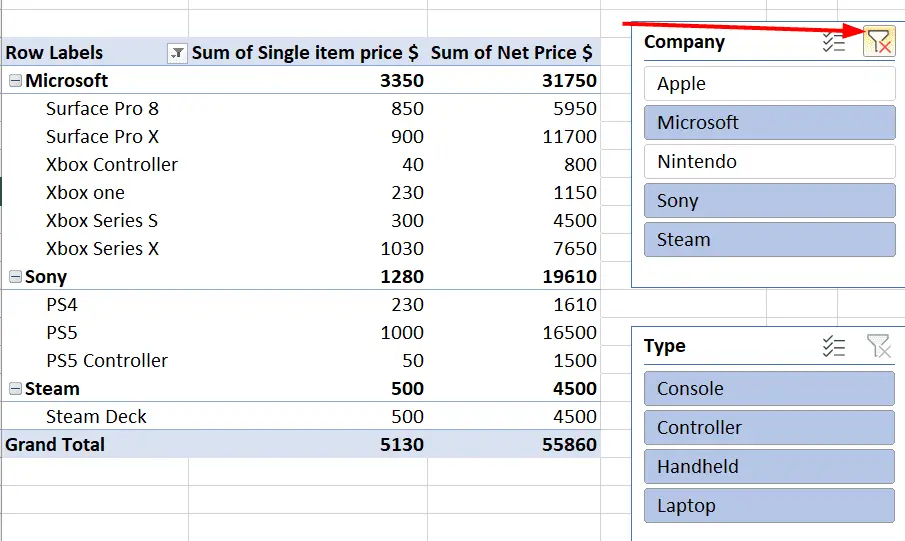
This is how, we can use Slicer to our advantage. It makes the the filtering of data easier by showing exactly what data is being shown and what is being filtered.
Related:

