

In this tutorial, we will learn how to use IFS function in excel. IFS function checks whether one or more conditions are true, and returns a value on a first corresponding True condition. IFS function can be used in the place for nested IF functions. Rather than using multiple if functions, IFS function can be used. Microsoft Excel 2021 is used.
In the arguments of the IFS function, first we write the logical condition and then the result for if the condition is true, otherwise, the next condition is checked and so on.
Syntax
=IFS( logical test 1, [value if true 1], logical test 2, [value if true 2], ...)
To specify a result for which none of the conditions are true, enter True in the final logical condition argument and then enter the value.
Up to 127 conditions can be checked.
For this tutorial, we will use example of a Grading system based on the marks of the students.
Following grade scheme will be implemented:
| Marks | Grade |
| > 90 | A+ |
| > 80 | A |
| > 70 | B |
| > 60 | C |
| > 50 | D |
| < 50 | F |
Using IFS function to make a Grading system
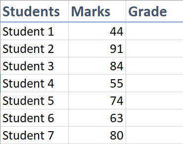
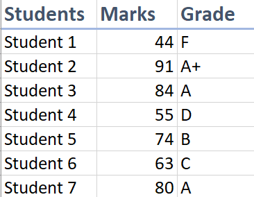
We will be using the following data.

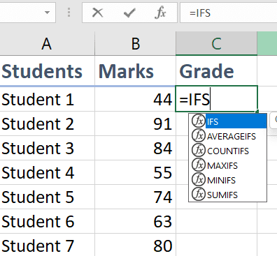
Type the function, in the cell, to start a function or formula, first put = sign, and the name of the function IFS.

Type the cell, for which the marks are to be compared. Enter the logical condition, B2>=90, "A+". Comma is used to separate the logical condition from value if the condition is true.

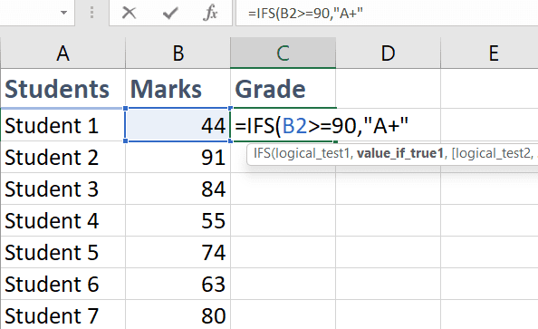
This means that if the marks are equal to or greater than 90, then the value of the cell will be “A+”.
Similarly, enter all the logical conditions and the values.
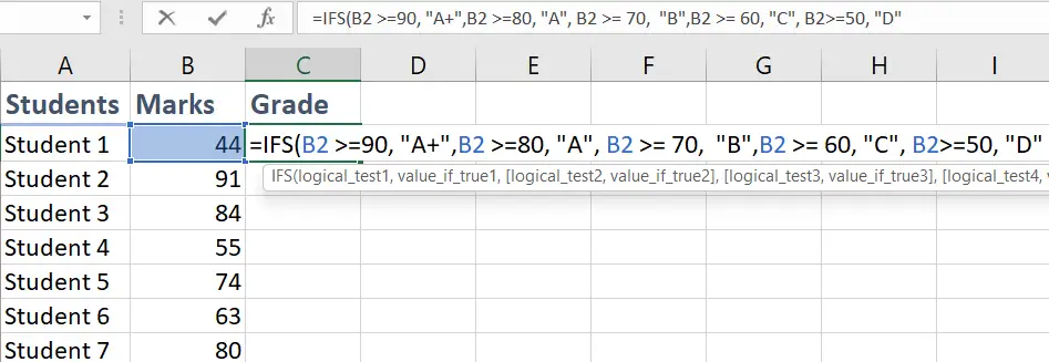
These are the grade criteria using IFS function. The value will be returned based on the value of the cells in the Marks column.
Now, we need to enter a default value, if none of the condition is true.
We enter True after all the logical conditions and their values, and then the default value, in this case, "F".
So, the formula becomes: =IFS(B2 >=90, "A+", B2 >=80, "A", B2 >= 70, "B",B2 >= 60, "C", B2>=50, "D",True, "F")

After completing the formula, we can apply this along the column, be selecting the cell, and then press and hold Left Mouse Button on the bottom right corner of the cell and drag along the column.
Check out more: How to use IF function.