

Pivot tables are used for organising and summarising data. They are used to point out the specific terms in an extensive data. Using Pivot tables, we can save a lot of time. Microsoft Excel 2021 is used.
In this tutorial, you will learn how to create a Pivot Table, click here if you want to know What is a Pivot Table.
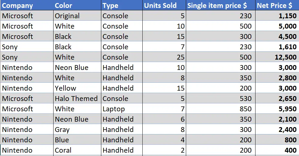
For this tutorial, we will take an example of a store that sells Laptops, gaming consoles, handheld gaming consoles and their accessories.
For each product, we have the following specifications.
- Company Name
- Color
- Type
- Units Sold
- Single item price
- Net price

Using this data, we will see how can we make this data more concise using PivotTable.
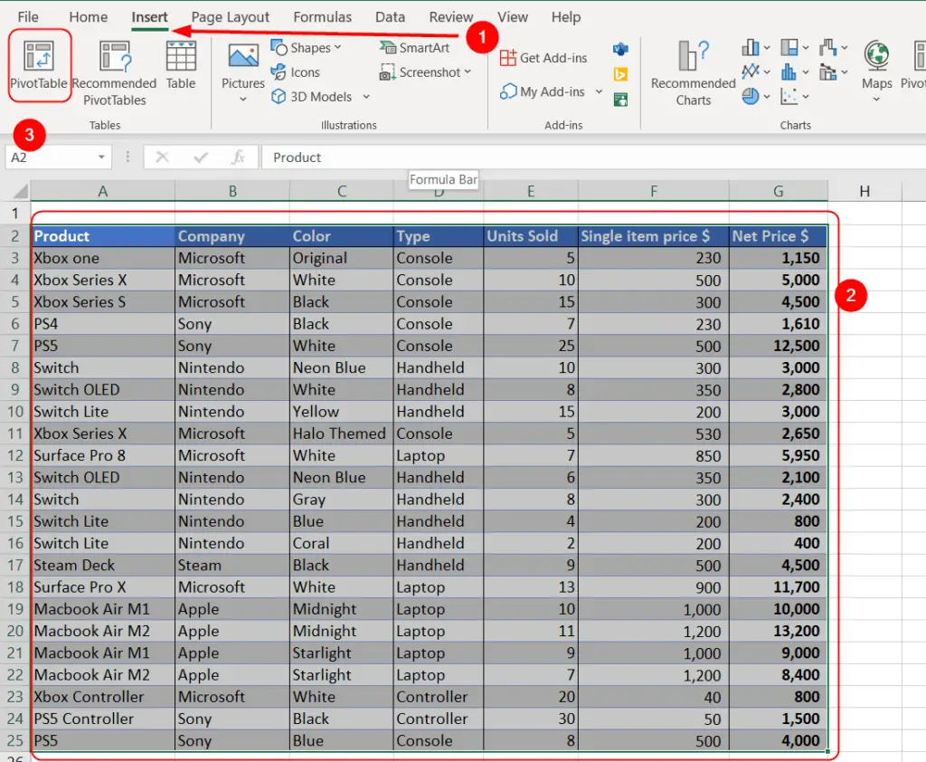
The data presented in this tutorial is a cell range, but a standard table can also be used.
To create a PivotTable, go to Insert tab from the top ribbon, select the Range, and then click PivotTable.

By clicking this, Create PivotTable menu will open, the Table/Range shall already be specified since you already selected the range for the PivotTable, in this tutorial, we are going to select New Worksheet for the PivotTable.

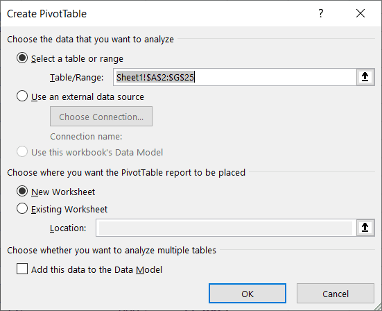
You can make a PivotTable using External Data source, but for this tutorial, we will use the current Range. For Multiple Tables, we may add the data to the Data Model but we will not be using this in this tutorial.
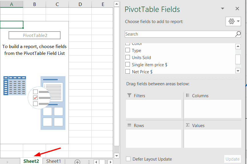
Making PivotTable report
The PivotTable will open in a new Worksheet.

Adding Fields to Areas
The PivotTables have Fields and Areas. To make a PivotTable report, we drag the Fields into the Areas.
There are four areas:
- Rows and Columns: This is the data we want to be shown, the primary data is put in Rows while the values such as Sum is shown in columns.
- Values: These are the Sum, Average, Count and other mathematical functions.
- Filters: This can be used to filter the data that is not needed.
Start by putting the Fields into the Rows. These are the fields for which you want to check other Fields such as the Price of Products.

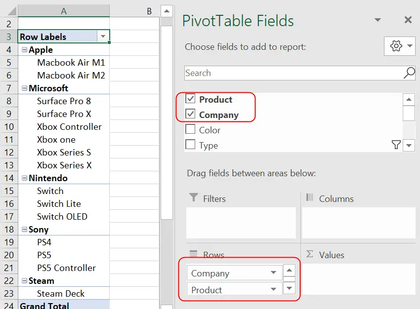
Note that, the Fields should be in Categorical order when they are added to Rows or Columns. The field that is put after becomes sub category.
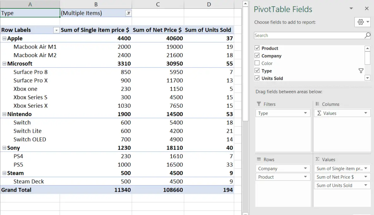
Next, we we will compare the prices of the products, so, we add price of Single item and Net price to the Value. So, drag the Fields in to Values area.

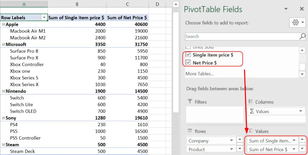
The Values area can perform mathematical operations such as Sum, Count, Average and more. Consequently, the Values parameter is added to Columns area.
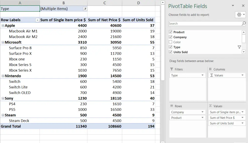
Adding Filters
Next, we can apply filter, so that only a specific type of data is available to us. Add the desired field to the Filters Area.

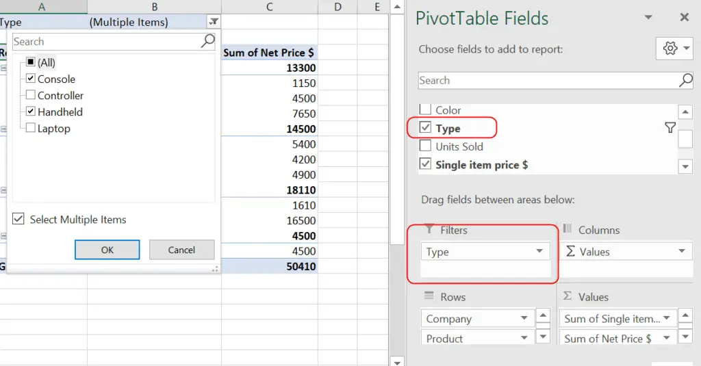
As it can be seen that we have made a PivotTable. This table can be sorted, summarized or it can be expanded depending on the requirement.

More on Pivot Table:
One reply on “Create a Pivot Table in Excel”
[…] To make a PivotChart, we need to have a PivotTable first, click here to learn about PivotTable. […]